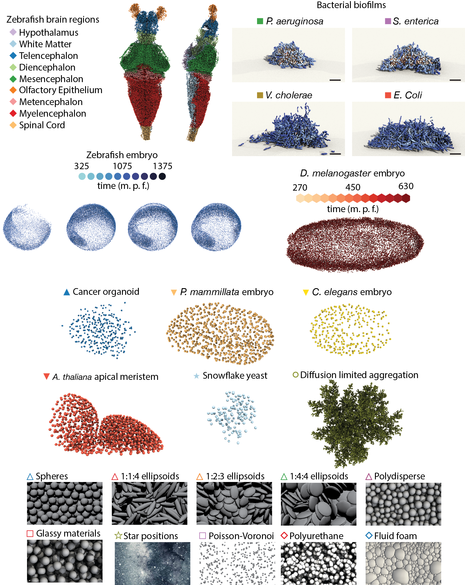
This interactive topological atlas shows a 3D Euclidean embedding of the pairwise topological distance matrix between various biological and physical systems, using multidimensional scaling (MDS). The topological distance computation relies only on local structural information contained in the Delaunay tessellations of 3D point clouds, which can represent particle centroids of a colloidal packing or nuclei position in tissues or cells in bacterial biofilms. Details of the distance definition and algorithms are described in Skinner, Jeckel, Martin, Drescher, and Dunkel Sci. Adv. (2023)
Select systems from the table below to explore different parts of the atlas. For every new selection the MDS embedding is recalculated. To contribute and help expand the atlas, please see instructions below.
| System name | Number of samples | Number of points per sample (approximate) | Data source |
|---|

References
[1] Ding et al., eLife, 8:e44898 (2019)
[2] Jeckel et al., bioRxiv:2021.08.06.4554
[3] Keller, Schmidt, Wittbrodt, and Stelzer, Science, 322:5904 (2008)
[4] Keller et al., Nat. Meth. 7:637 (2010)
[5] Cao et al., Nat. Commun. 11:6254 (2020)
[6] Guignard et al., Science 369:eaar5663 (2020)
[7] Han et al., Nat. Phys. 16:101 (2020)
[8] Donev, Torquato, and Stillinger, J. Comput. Phys. (2005)
[9] Bapst et al., Nat. Phys., 16:448 (2020)
[10] The HYG Database
[11] Willis et al., Proc. Natl. Acad. Sci. USA, 113:E8238 (2016)
[12] Bogunia, Buchen, and Weinberg, GAMM-Mitteilungen, 45:e202200018 (2022)
[13] Karnakov, Litvinov, and Koumoutsakos, Sci. Advan., 8:eabm0590 (2022)
[14] Day et al., eLife, 11:e72707 (2022)
This website was built and is maintained by Dominic J. Skinner
Contributing to the atlas
To contribute a system to expand the atlas, you will need to provide the following:
1. Files of the format "system_name_exp_1.csv", "system_name_exp_2.csv", etc., with the first row as "x, y, z" and subsequent rows containing the x, y, z, values of points in the system.
2. If the system is not periodic, provide an appropriate radius for the alpha complex to identify the edge points. The matlab script at the bottom of this page can help identify an appropriate radius.
3. (optional) A representative image of the system to add to the legend.
4. The way in which you would like to be cited.
Send the above information to topological.atlas.contribute@gmail.com
Below is an example matlab script that can be run to find an appropriate alpha radius for your system. The radius should be set large enough as to only identify points on the boundary of your system.
    csv_input_file = 'path/to/formatted_file.csv';
    vertices = table2array(readtable(csv_input_file));
    simplices = delaunay(vertices);
    a_vals = alpha_shape3D(simplices,vertices);

    edge_vals = [];
    alpha_val = 2*median(a_vals); %a good starting point, but adjust as necessary
    for i = 1:length(a_vals)
        if a_vals(i) > alpha_val
            edge_vals = [edge_vals; simplices(i,:)];
        end
    end
    edge_vals = unique(edge_vals);

    scatter3(vertices(:,1),vertices(:,2),vertices(:,3))
    hold on
    scatter3(vertices(edge_vals,1),vertices(edge_vals,2),vertices(edge_vals,3))
    % points identified as boundary points will appear in orange

    % Helper functions below
    function r = circumradius3D(e1,e2,e3,e4)
        e_n = [norm(e1)^2 ; norm(e2)^2; norm(e3)^2; norm(e4)^2];
        e_mat = [e1 1 ;e2 1 ;e3 1 ;e4 1];
        e_mat = [e_n e_mat];
        a = det(e_mat(:,2:5) );
        Dx = det(e_mat(:,[1, 3:5]));
        Dy = det(e_mat(:,[1:2, 4:5]));
        Dz = det(e_mat(:,[1:3, 5]));
        c = det(e_mat(:,1:4));
        r = Dx^2+Dy^2+Dz^2-4*a*c;
        if r >= 0
            r = sqrt(r)/(2*abs(a));
        else
            r = Inf;
        end
    end

    function a_val = alpha_shape3D(simplices,p)
        a_val = zeros(length(simplices(:,1)),1);
        for s = 1:length(simplices(:,1))
            e1 = p(simplices(s,1),:);
            e2 = p(simplices(s,2),:);
            e3 = p(simplices(s,3),:);
            e4 = p(simplices(s,4),:);
            a_val(s) = circumradius3D(e1,e2,e3,e4);
        end
    end